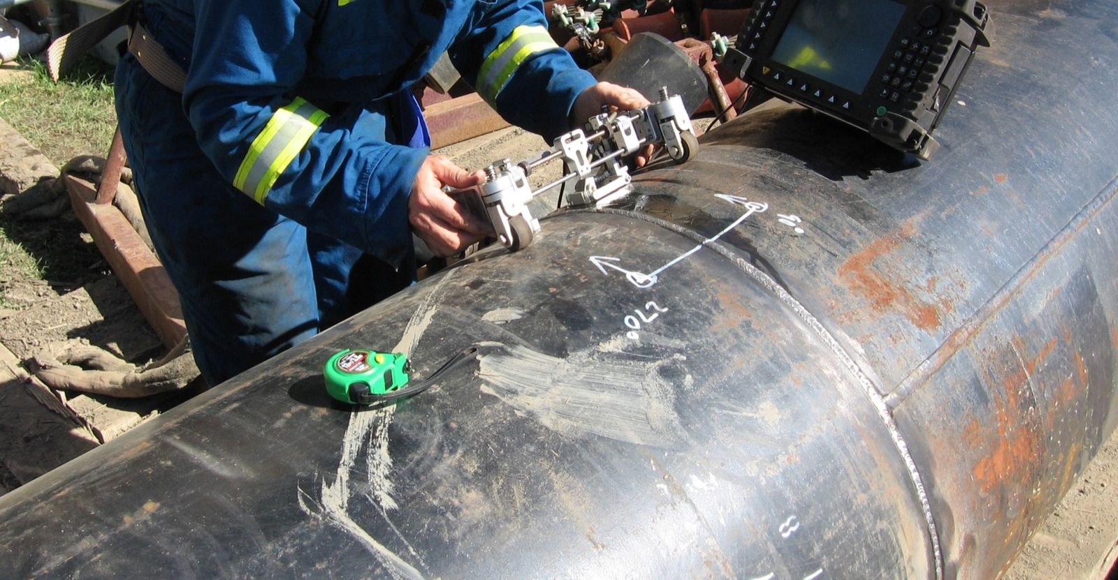
In the maintenance of oil & gas, chemical, power and marine plants, most recurring NDT work is about following wall loss rather than hunting for manufacturing flaws. Internal corrosion, erosion, corrosion under insulation, localized attack downstream of an injection point: different mechanisms that all end up in one measurable parameter, the remaining wall thickness. An ultrasonic thickness gauge measures it from one side, in a few seconds, without stopping operation and without removing material.
Getting a number is easy, since any instrument will display one. The real work starts when that number has to be correct, repeatable and comparable with the one taken four years ago, because the engineering value lies in the time series used to calculate corrosion rate and remaining life. That series is where a poorly chosen or poorly used gauge does the most damage, with plausible readings that are wrong in the same direction for years.
The instrument measures time, and velocity decides the rest
An ultrasonic thickness gauge works in pulse-echo mode: the probe emits a short longitudinal pulse that crosses the wall, reflects off the opposite surface and returns to the receiver. The instrument measures the time of flight tf and calculates thickness s as s = v · tf / 2, where v is the longitudinal wave velocity in the material and the factor 2 accounts for the round trip.
The practical consequence needs to be clear: the instrument doesn't measure a thickness, it measures a time. All of the accuracy depends on the velocity setting, and a 2% velocity error becomes a 2% thickness error. On a 10 mm wall that is 0.2 mm, the same order of magnitude as the loss a corrosion survey is meant to detect.
The velocities in the table are indicative values from the industry's standard reference tables and serve as a starting point. Composition, heat treatment, grain structure, rolling direction and temperature shift them, which is why both ISO 16809 and ASTM E797 call for calibration on a sample of the same material.
| Material | Indicative longitudinal velocity | Notes |
|---|---|---|
| Carbon steel | ≈ 5900 m/s | Reference value for most corrosion applications |
| Austenitic stainless steel (304/316) | ≈ 5660-5740 m/s | Anisotropic structure: take care with castings and weld deposits |
| Aluminum | ≈ 6300 m/s | Varies with alloy; recalibrate for structural alloys |
| Titanium and alloys | ≈ 6000-6100 m/s | Alloy dependent |
| Copper | ≈ 4700 m/s | High attenuation at high frequencies |
| Brass | ≈ 4400 m/s | Strongly composition dependent |
| Cast iron | ≈ 3500-5600 m/s | Highly variable with graphite form and structure: calibration on the part is mandatory |
| Rigid PVC | ≈ 2400 m/s | Attenuating material: low frequencies |
Proper calibration has two parts. Zero compensates for electronic delay and transit through the delay line or probe shoes, and is set on the block supplied with the instrument. Velocity is derived on a step wedge of the same material and surface condition as the component. Two steps, one thin and one thick, bracketing the expected range correct zero and velocity together, and the result is far more reliable than single-point calibration. On an unknown material the procedure runs the other way, measuring a sample of the same material with a micrometer and deriving the velocity from the measured time.
Mode 1, Mode 2, echo-to-echo: what ends up in the number
The three classic modes differ in which echoes are used as time references, and therefore in what goes into the timed path. In Mode 1 a single-element contact probe measures the interval between the excitation pulse and the first backwall echo. It is the simplest option and works on clean, regular surfaces, but the probe's ring-down blinds the first microseconds and sets a lower thickness limit.
Mode 2 uses a delay line or a dual-element probe and times from the interface echo, the entry into the part, to the first backwall echo. Separating the excitation pulse from the measurement zone lets the gauge go much thinner and keeps the reading stable on irregular surfaces, which is why it is the usual mode for corrosion measurement with dual-element probes.
Mode 3, or echo-to-echo, measures the interval between two successive backwall echoes. The timed path lies entirely in the metal, so delay line, couplant and above all paint drop out of the count. This is what allows measurement through coatings without removing them, a considerable operational saving on painted lines. It comes at a price: it needs at least two clean, well-separated backwall echoes, so a reasonably regular back surface, a low-attenuation material and a thin, well-bonded coating. A wall heavily corroded on the far side scatters the beam and the second echo disappears; at that point the right move is to strip the coating locally and measure in Mode 2 rather than force an unstable reading.
In Mode 1 and Mode 2 on a painted surface, on the other hand, the coating enters the acoustic path. Its velocity is much lower than that of steel, and the reading is systematically overstated: a dangerous error, because it goes in the non-conservative direction.
Dual element or single element: the choice that matters most
A dual-element probe carries two separate crystals, one transmitting and one receiving, acoustically isolated and tilted at a small roof angle to the surface. Where the two beams cross there is a zone of maximum sensitivity at a certain depth, a kind of pseudo-focus that makes the measurement tolerant of rough, oxidized or corroded surfaces and irregular backwalls. It is the reference configuration for corrosion work, but it has limits worth knowing. Linearity worsens on very thin walls, the minimum measurable thickness is on the order of a millimeter for 5 MHz probes, component curvature disturbs the reading and minimum thicknesses need V-path correction.
A single-element probe with a delay line, usually at a higher frequency (7.5-15 MHz), offers better linearity and resolution on small thicknesses. It is the choice for thin walls, heat exchanger tubes, machined parts and precision measurements, where dual-element probes can't reach. The practical rule stays simple: dual element for corrosion, single element with a delay line for thin walls and precision. Anyone inspecting both process lines and tube bundles therefore needs an instrument that accepts both probe families.
There are also high-temperature dual-element probes, with heat-resistant delay lines and dedicated couplants, to be used for brief contact and within the temperature limits stated by the probe manufacturer. They only work inside a procedure: short contact, cooling between readings and velocity correction, discussed further on.
Errors that repeat until the cause is removed
Ultrasonic thickness measurement errors are almost all systematic, and that is what makes them insidious: they recur identically at every survey and build a trend that is false but consistent. The table collects the most frequent ones in the field.
| Error | Physical cause | Countermeasure |
|---|---|---|
| Doubling (double or multiple reading) | The instrument fails to resolve the first backwall echo and locks onto the second | Stay within the probe's range; switch to a high-frequency single element; distrust readings exactly twice the expected value; always check the A-scan |
| Overstated reading on a painted surface | The low-velocity coating enters the path in Mode 1/2 | Echo-to-echo mode (Mode 3) or local coating removal |
| Overstated reading on a hot component | Sound velocity in steel decreases as temperature rises | Correction of about −1% per 55 °C (100 °F) above calibration temperature for carbon steel, or calibration on a block brought to the same temperature |
| Lost echo or understated value on pitting | The concave, irregular pit bottom scatters the beam | Focused dual element, higher frequency, slow scanning for the minimum, encoded scanning when pitting governs the assessment |
| Anomalous reading on laminations, inclusions, hydrogen blistering | An intermediate reflector is taken for the backwall | Watch the A-scan shape, compare with surrounding points, don't trust the number alone |
| Unstable or missing readings | Poor coupling, mill scale, flaking rust, corrosion products | Mechanical surface preparation, couplant viscosity suited to roughness and temperature, constant contact pressure |
| Error on small diameters | Partial probe contact on the curved surface | Suitable probe diameter, contoured delay line, crystals oriented perpendicular to the pipe axis |
| Calibration drift during the shift | Delay line wear, probe temperature change | Check zero and velocity at the start and end of each session and at every change of probe, material or operator |
Almost every row in the table can be recognized from the shape of the signal. A gauge with an A-scan is the diagnostic tool that tells a valid reading from doubling, a lamination echo or poor coupling. A display that shows only the number, by contrast, gives no way of knowing why the number is what it is. In an inspection program built on trends, a false reading does more harm than a missing one.
Temperature deserves precision, because in a plant it is the most underestimated error. The velocity of ultrasound in steel falls as temperature rises. ASTM E797/E797M-21 applies to measurements up to 93 °C and indicates, for carbon steel, a correction on the order of −1% per 55 °C (100 °F) of deviation from the calibration temperature. Beyond that limit dedicated probes and procedures are needed. The exact dependence varies with composition, as shown by the experimental study of ultrasonic velocity and attenuation in low-carbon steel at high temperature. On critical hot lines, a generic coefficient is therefore worth less than calibration on a block of the same material brought to operating temperature.
Need thickness readings set up or made comparable?
Tell us the material, thickness range, temperature, coatings and number of CMLs: we propose a suitable probe, mode and data logging and test them on your component.
Email us Message us on WhatsAppWhat to look at when choosing a thickness gauge
The first criterion is measuring range together with resolution: 0.1 mm is enough to follow general corrosion, 0.01 mm is needed where precision and fine changes matter. The useful range also depends on the instrument-probe pair. On frequency the choice follows the material. 2.25 MHz suits attenuating or coarse-grained materials such as cast iron, castings and plastics, and heavy walls. 5 MHz is the general choice for corrosion on steel, while 7.5-10 MHz serves thin walls, small diameters and better resolution on pitting.
If you have to measure on painted surfaces that can't be prepared, echo-to-echo mode is a requirement to write into the order. Alongside the A-scan, a B-scan returns the thickness profile along a manual scan and is the cheapest way to find the minimum that a fixed-point grid can miss. The data logger does the rest: preloaded CML grids, unique point identification, threshold alarms and export to the inspection database turn a collection of numbers into a traceable program.
Then come the environmental requirements. Where lines can't be shut down, high-temperature probes and couplants are needed; in the field, IP65 or IP67 protection, drop resistance, display readability outdoors and battery life covering a full shift all count. In the classified areas of refineries, petrochemical plants and storage terminals, ATEX or IECEx certification is a blocking requirement and must be checked before any technical trial. And certified step wedges in the materials of interest are as much part of the supply as the probe.
When a single point is no longer enough
A thickness gauge samples: it measures where the probe is placed. If the damage is general and fairly uniform corrosion, the sample is representative and measurement at fixed CMLs remains the right, economical method. If the damage is localized, such as pitting, erosion on the outside of a bend, preferential attack of the heat-affected zone or corrosion under insulation, the chance that the grid hits the actual minimum is low. And the minimum is exactly the value that governs remaining life.
That is where encoded scanning comes in, returning a continuous thickness map instead of a list of points and supplying the input data for a fitness-for-service assessment to API 579-1/ASME FFS-1. How such a campaign is organized, what data density it needs and when it really pays off is explained in the article on ultrasonic corrosion mapping. The phased array technique it usually relies on is described in the PAUT guide. The two measurements work together: the gauge follows the CMLs over time, and mapping steps in when a point drifts off trend or a thin area needs sizing.
The standards that make a measurement defensible
The method reference is ISO 16809:2025, which sets the principles of ultrasonic thickness measurement by contact and immersion, calibration and influencing factors, adopted in Europe as EN ISO 16809:2025. On the US side, ASTM E797/E797M-21 covers manual pulse-echo contact measurement, with the range up to 93 °C and guidance on temperature correction.
Who performs the measurement is the second link. ISO 9712:2021 governs qualification and certification of NDT personnel by method. When the code or the client requires it, in-service thickness measurement must be performed by personnel certified for the UT method, following the organization's written procedure. Then come the in-service codes that use those numbers. API 570 for piping, API 510 for pressure vessels and API 653 for storage tanks define CML logic, rate calculations and inspection intervals. Downstream, API 579-1/ASME FFS-1 is used to assess wall loss. ASME Section V collects the general ultrasonic examination requirements referenced by construction and repair codes.
From the number to the inspection plan: CMLs, corrosion rate, remaining life
A CML (Condition Monitoring Location, formerly TML) is a fixed, identified, marked and repeatable position measured at every survey. An inspection program owes more to where the CMLs are placed than to the precision of the instrument. Priority goes to the outside of bends, tees and reducers, sections downstream of injection and mixing points, stagnant zones, low points where free water can collect, welds with their heat-affected zones and areas under insulation. For each CML the lowest reading in the examined area is recorded, or the average of several readings if the procedure says so, always with the same method, probe and mode.
Two rates are calculated from those readings. The long-term rate is CRLT = (tinitial − tactual) / years elapsed, and the short-term rate is CRST = (tprevious − tactual) / years between the last two readings. Remaining life is (tactual − tmin) / rate, with tmin the minimum required thickness from the design calculation. The more conservative of the two rates is used: if the short-term rate is higher, the damage mechanism has accelerated and scheduling must follow the worse figure. The interval to the next measurement is then set at the lesser of half the remaining life and the maximum interval allowed by the applicable code.
An example makes the numbers concrete. A DN 150 Sch 40 carbon steel process line, nominal wall 7.11 mm, minimum thickness from calculation 4.80 mm, in service since 2006. CML 07 has two readings, 6.40 mm in 2022 and 5.80 mm in 2026.
- CRLT = (7.11 − 5.80) / 20 years = 0.066 mm/year
- CRST = (6.40 − 5.80) / 4 years = 0.150 mm/year, which becomes the governing rate
- Remaining life = (5.80 − 4.80) / 0.150 = 6.7 years
- Interval to the next measurement = half the remaining life, about 3.3 years: scheduled at 3 years, if below the code maximum
A short-term rate that jumps above the history signals a change of regime. It may come from a process change, free water or a temperature shift, and it calls for an investigation of the cause as well as a shorter interval.
What to send us for an assessment
To propose the right gauge configuration we need a few data points:
- material and surface condition, with presence and type of coating;
- expected thickness range and minimum pipe diameters;
- operating temperature at the points to be measured;
- prevailing damage mechanism, general or localized;
- number of CMLs and inspection database or software in use;
- ATEX classification of the areas and personnel certification requirements.
You can send them by email to info@dipitech.com or on WhatsApp, attaching your latest thickness readings if you have them.
With this data the configuration can be defined in full: probe or probe set, measurement mode, data logging functions, reference blocks and operator training, with a test on the real component and a comparison between operators on repeatability. Where a single point isn't enough, the assessment extends to the scanning and mapping instruments on the page for PAUT and TOFD ultrasonic instruments.
Request a quote
Leave your name, email, and a few lines about your application, with no obligation. We reply within 24 hours with initial technical guidance and a quote.
Frequently asked questions about ultrasonic thickness gauges
What is an ultrasonic thickness gauge used for?
It measures the remaining wall thickness from one side only, in a few seconds, without stopping operation or removing material. In the maintenance of piping, pressure vessels and storage tanks it is the instrument used to track wall loss from corrosion and erosion. Repeated readings at the same condition monitoring locations (CMLs) build the history from which corrosion rate and remaining life are calculated.
How does an ultrasonic thickness gauge work?
The probe sends a short ultrasonic pulse that crosses the wall, reflects off the opposite surface and travels back. The instrument measures the time of flight and derives thickness by multiplying it by the sound velocity in the material and dividing by two, because the path runs out and back. That is why accuracy depends on velocity calibration on a block of the same material: a 2% error in velocity becomes a 2% error in thickness.
How much does an ultrasonic thickness gauge cost?
There is no single price, because the figure changes with the instrument class and above all with what is really needed: A-scan, echo-to-echo mode, data logger with CML grids, interchangeable probes, ATEX certification, reference blocks. An instrument bought without the function you need ends up being paid for twice. DIPITECH helps you choose new instruments and prepares a tailored quote within 24 hours based on the material, thicknesses, temperature and coatings of the application.
Can thickness be measured through paint or coating?
Yes, in echo-to-echo mode, provided the coating is thin and well bonded and the backwall returns at least two clean echoes. A quick field check is to measure the same point twice: in echo-to-echo and then, after stripping the paint locally, in Mode 2. If the two readings agree within the procedure's tolerance, echo-to-echo is reliable on that line and can be used for later surveys.
Can a thickness gauge be used on heat exchanger tubes?
Yes, from the outside and where the tube is accessible, with a high-frequency single-element probe and a delay line contoured to the diameter. To inspect a tube bundle from the inside, tube by tube, other techniques are used, such as remote visual inspection with a videoscope, eddy current or rotating ultrasonic probes. The gauge remains useful for spot-checking thickness in reachable areas.
How often should an ultrasonic thickness gauge be recalibrated?
The operational check of zero and velocity is done at the start of each session and at every change of material, probe, operator or significant temperature. Periodic laboratory calibration with traceable blocks follows the quality system interval, often annual. The detail that gets overlooked is that reference blocks also carry a certificate, and a block without one makes the calibration performed on it worthless.
What is the minimum measurable thickness, and what is doubling?
The minimum depends on the probe-mode pair: a 5 MHz dual-element corrosion probe is reliable from about a millimeter upward, while a high-frequency single element with a delay line goes considerably lower. Below the limit doubling appears, a reading about twice the real thickness. The typical warning sign is a thin wall that suddenly reads thicker than nominal: it should always be checked on the A-scan.